| 5.1 | Address - Triad Element 1 |
| 5.2 | Route - Triad Element 2 |
| 5.3 | Rule - Triad Element 3 |
| 5.4 | Cisco Policy Routing Example |
| 5.5 | RPDB & Multiple Route Tables |
| 5.6 | All Together Now |
| 5.7 | Summary |
This chapter will take you through a series of implementation examples for Policy Routing. These examples primarily draw upon the use and configuration of Policy Routing under Linux. You will see the various uses of the ip utility, which was illustrated in Chapter 4. In some instances I will use and refer to other utilities and methods for configuring the structure but will not be explaining those utilities in this book.
This chapter starts off with the Policy Routing core subjects of addresses, routes, and rules. As you saw in Chapter 3, these subjects comprise the core of the RPDB. In most cases I start with the overall theory and delve deeper into the ramifications of implementing that theory. Interspersed throughout are practical examples intended to reinforce the theory and usage. The examples create an ever-increasing complexity and illustrate many of the concepts of Policy Routing. You will see how the limitations of the protocols come into play especially when considering implementations within a finite network structure.
After covering the fundamentals of addressing, routes, and rules, you will jump into the interactions and manipulation of multiple routing tables. This covers the more esoteric structures using tables with some simple rule structures. Then all of the basics are applied to illustrate the complex interactions that can be created with simple steps. In this scenario you will explore the full gamut of addressing, routes, and rules all multiply interacting. At the end of this chapter you will have full control of the basics, a black belt of Policy Routing in Linux.
The first and most basic of the Policy Routing structure elements is the addressing structure. This fundamental part of an IP network is often completely taken for granted. In the many sessions I have given on using Policy Routing in Linux, I am always asked why I even bother discussing addresses. In reply, I usually ask if anybody there can explain what an IP address is. With your own answer to this question in mind, let me begin.
When looking at a Policy Routing setup you should start by considering the IP addressing structure. The use and interactions of addressing in an IPv4 network often indicate the fundamental data flow of the network structure. To fully understand how these addresses interact with the routing structure of the network, I will first discuss some of the theory of addressing under IPv4 with some forward references to IPv6 as well. From this basis you can see why some of the problems within routed networks currently exist.
5.1.1 Fundamental IP Address Concepts
The fundamental design notion behind IPv4 addresses is that an address uniquely identifies the source of a set of services. Most people consider an IP address as identifying a single network interface on a particular machine. But that is a misperception of the address. Think deeper of the actual sequence of events defining how you would locate a given address on a particular network segment.
When considering the communication on a given physical network, say an Ethernet or Token Ring hub, under IPv4 the IP address is not used in direct communication. Any two network devices under IPv4 communicate over a physical network using their respective Media Access Control (MAC) addresses. This is the reason behind Address Resolution Protocol (ARP). On any physical network you can have as many different IPv4 networks as you want coexistent and unaware of each other. Under such a network scheme you may talk of routing structures required between two machines on the same physical network.
A physical network structure that has coexistent, independent IPv4 networks defined and operational provides a good perspective for understanding the divorce of addressing from physical structure. In those conditions you may have multiple complete IPv4 networks defined as matching identical MAC addresses. When you communicate under such a network setup you use the IP address that is appropriate for the network you want to communicate with. Consider the following information and setup:
| Machine A - eth0: | MAC Address - 00:11:22:33:44:AA | IP Address - 192.168.1.1/24 |
| Machine B - eth0: | MAC Address - 00:11:22:33:44:BB | IP Address - 10.1.1.1/8 |
| Machine C - eth0: | MAC Address - 00:11:22:33:44:CC | IP address - 192.168.1.254/24, 10.254.254.254/8 |
Since Machine C has two IP addresses assigned it is probably the router. Now look at the arp tables on Machine A and Machine B and you will see two different IP addresses associated with the same MAC address. Machine A's arp table lists IP address 192.168.1.254 as having MAC address 00:11:22:33:44:CC and Machine B's arp table lists IP address 10.254.254.254 as having MAC address 00:11:22:33:44:CC.
By seeing the IP address as simply a pointer to the location of a set of services you can see why many of the tricks of IP become a normal conclusion. For a more detailed discussion of this structure I recommend you read RFC-2101. Spoofing, loopback, and hijacking, along with load balancing, proxy ARP, and NAT, are all functions of the "free" nature of IPv4 addresses.
Consider how you match up a human-readable network name such as www.policyrouting.org with the associated IPv4 address. The DNS service provides a correlation between these two items. Then when you want to see what information is available under the http protocol on that network node, your browser queries the IP address returned from the DNS lookup with a specific request for the "well-known" service port. In this case the IP address is providing a reference platform for obtaining the service. But what is that reference platform?
Now the notion that an IP address is associated with a particular interface becomes hazardous. When you consider what reference platform is associated with the IP address you must take into account the fact that there is no reliable association of the IP address to any particular physical system. Indeed, if the http service considered here were behind a hardware load balancer, the notion of that IP address as "belonging" to any particular hardware system is ludicrous. The only definition of the service relies on the provision of many systems feeding a common output.
Implausible and confusing as this may seem at first glance, the type of setup required to implement this scenario is all too familiar. Consider a standard NAT firewall or any IPv4 load balancing system and you will see that the IP addressing mechanisms are used to define a service without reference to any physical interface. When I speak of an IP address, then, I refer to the services and usage of that address and not to any particular physical manifestation of that address.
Now that an IP address no longer belongs to a physical interface you can start to look at the various methods of using it. This is where you start to play with the IP address structure of the network. By defining the IP address structure you can implement additional methods of Policy Routing.
Example 5.1.1 - Multiple IP Addressing
The following exercise in implementing multiple IP addresses will help you further understand the parts of the IP address functions. This hands-on exercise will then be used as the basis for the rest of the addressing structure explanations.
You will create multiple IP addresses and explore several of the additional device structures provided under Linux. All of the features are available under Kernel 2.1.32 or higher. The utility is ip from the IPROUTE2 package.
Your machine has two network interface cards (NICs) installed. One is Ethernet (eth0) and the other is TokenRing (tr0). Additionally you have the Dummy, Tap, and several flavors of Tunnel interface. You start with no addresses configured with the lone exception of loopback. So your system output from ip addr list would look as follows:
1: lo: <LOOPBACK,UP> mtu 3924 qdisc noqueue
link/loopback 00:00:00:00:00:00 brd 00:00:00:00:00:00
inet 127.0.0.1/8 brd 127.255.255.255 scope host lo
inet6 ::1/128 scope host
2: dummy: <BROADCAST,NOARP> mtu 1500 qdisc noop
link/ether 00:00:00:00:00:00 brd ff:ff:ff:ff:ff:ff
3: eth0: <BROADCAST,MULTICAST,UP> mtu 1500 qdisc pfifo_fast qlen 100
link/ether 00:11:22:33:44:aa brd ff:ff:ff:ff:ff:ff
inet6 fe80::211:22ff:fe33:44aa/10 scope link
4: tr0: <BROADCAST,MULTICAST,UP> mtu 2000 qdisc pfifo_fast qlen 100
link/ether 00:11:22:33:44:bb brd ff:ff:ff:ff:ff:ff
inet6 fe80::211:22ff:fe33:44bb/10 scope link
5: tap0: <BROADCAST,MULTICAST,NOARP> mtu 1500 qdisc noop
link/ether fe:fd:00:00:00:00 brd ff:ff:ff:ff:ff:ff
6: tunl0@NONE: <NOARP> mtu 1480 qdisc noop
link/ipip 0.0.0.0 brd 0.0.0.0
7: gre0@NONE: <NOARP> mtu 1476 qdisc noop
link/gre 0.0.0.0 brd 0.0.0.0
8: sit0@NONE: <NOARP> mtu 1480 qdisc noop
link/sit 0.0.0.0 brd 0.0.0.0
9: teql0: <NOARP> mtu 1500 qdisc noop qlen 100
link/generic
Now you will configure your eth0 interface to have three IPv4 addresses: 10.1.1.1/8, 172.16.1.1/16, and 192.168.1.1/24. Your tr0 interface will have the following three addresses: 10.1.1.2/8, 172.16.1.2/16, and 192.168.1.2/24. This is accomplished through the following command sequence:
ip addr add 10.1.1.1/8 dev eth0 brd +
ip addr add 172.16.1.1/16 dev eth0 brd +
ip addr add 192.168.1.1/24 dev eth0 brd +
ip addr add 10.1.1.2/8 dev tr0 brd +
ip addr add 172.16.1.2/16 dev tr0 brd +
ip addr add 192.168.1.2/24 dev tr0 brd +
Now that you have installed the addresses you should have output similar to this from ip addr list:
1: lo: <LOOPBACK,UP> mtu 3924 qdisc noqueue
link/loopback 00:00:00:00:00:00 brd 00:00:00:00:00:00
inet 127.0.0.1/8 brd 127.255.255.255 scope host lo
inet6 ::1/128 scope host
2: dummy: <BROADCAST,NOARP> mtu 1500 qdisc noop
link/ether 00:00:00:00:00:00 brd ff:ff:ff:ff:ff:ff
3: eth0: <BROADCAST,MULTICAST,UP> mtu 1500 qdisc pfifo_fast qlen 100
link/ether 00:11:22:33:44:aa brd ff:ff:ff:ff:ff:ff
inet 10.1.1.1/8 brd 10.255.255.255 scope global eth0
inet 172.16.1.1/16 brd 172.16.255.255 scope global eth0
inet 192.168.1.1/24 brd 192.168.1.255 scope global eth0
inet6 fe80::211:22ff:fe33:44aa/10 scope link
4: tr0: <BROADCAST,MULTICAST,UP> mtu 2000 qdisc pfifo_fast qlen 100
link/ether 00:11:22:33:44:bb brd ff:ff:ff:ff:ff:ff
inet 10.1.1.2/8 brd 10.255.255.255 scope global tr0
inet 172.16.1.2/16 brd 172.16.255.255 scope global tr0
inet 192.168.1.2/24 brd 192.168.1.255 scope global tr0
inet6 fe80::211:22ff:fe33:44bb/10 scope link
5: tap0: <BROADCAST,MULTICAST,NOARP> mtu 1500 qdisc noop
link/ether fe:fd:00:00:00:00 brd ff:ff:ff:ff:ff:ff
6: tunl0@NONE: <NOARP> mtu 1480 qdisc noop
link/ipip 0.0.0.0 brd 0.0.0.0
7: gre0@NONE: <NOARP> mtu 1476 qdisc noop
link/gre 0.0.0.0 brd 0.0.0.0
8: sit0@NONE: <NOARP> mtu 1480 qdisc noop
link/sit 0.0.0.0 brd 0.0.0.0
9: teql0: <NOARP> mtu 1500 qdisc noop qlen 100
link/generic
You may recall the various items of information in this printout from the discussion of the ip utility in Chapter 4. An important one is the definition of the addresses on the inet lines. For example, the eth0 address 10.1.1.1/8 has a scope global toward the end of the line. This scope parameter is the second important topic of IP addressing.
Many operating systems have methods of assigning multiple IP addresses to an interface. These multiple assignments often code the assignment in terms of fragmented interfaces. A fragmented interface, often referred to as a coloned interface often referred to as an IP alias for those of you running most Linux Distributions, is a subinterface defined as a virtual part of the primary interface. You usually see these addresses and assignments in terms of being allocated one to one with a specific interface fragment. Recalling the multiple IP addresses from example 1 you would have seen that eth0 = 10.1.1.1/8, eth0:1 = 172.16.1.1/16, and eth0:2 = 192.168.1.1/24. This tying of the IP address to a virtual interface fragment violates the fundamental consideration of IP addresses being independent of assignment.
What sets the Policy Routing usage apart, especially under Linux, is the concept of addressing scopes. When you assign multiple IP addresses to a single interface under the fragmented interface setup, you treat the first entered address as the primary and the rest of the addresses as secondaries. If you delete the primary address the interface goes away and you lose all other addresses. The interface is paramount in this scenario.
In Policy Routing the treatment of IP addresses obeys the fundamental disassociation of address from physical assignment. Thus when you assign multiple IP addresses to an interface in Policy Routing, you have complete independence of the addresses. There is no fragmented interface to which the address is associated. Instead, all addresses are treated equal and capable of being used independently. However, this brings up the question of how an IP address is defined with respect to the IP network structure.
The definition of an IP address scope ties together the concept of the address and the network. An address exists independently of the network and other addresses. Defining which addresses fit into which network spaces is purely a matter of definition with respect to the IP address itself. This definition is coded through the Classless Inter Domain Routing (CIDR) mask value.
A CIDR mask specifies the masking bits used on an IP network. This is the subnet mask when referencing the network itself. In Policy Routing addressing, this mask specifies the scope of the address space by defining the network coverage. Thus when you have a CIDR mask of /24, you define a network originally referred to as a Class C network. The address scope is then defined as having that address being a member of that network.
This sounds convoluted but is very simple. An example should clarify this somewhat. Consider the addressing structure you implemented in Example 5.1.1. Each of the addresses in that example had an independent scope. Thus if you look at the addressing for eth0 from that example you have three scopes - call them A, B, and C.
| 10.1.1.1/8 | Scope A |
| 172.16.1.1/16 | Scope B |
| 192.168.1.1/24 | Scope C |
To show the extent of the scope, consider a simple quiz. Which of the following addresses below belong to which scope listed above?
10.1.1.2/16
172.16.1.2/24
192.168.1.2/24
The answers, in order, are: D (new), E (new), C. Both of the first two addresses and CIDR masks define new scopes, D & E. Only the last one is a member of a preexisting scope. Yes, 10.1.1.2 as an independent address can be considered as belonging to the range of addresses defined by 10.1.1.1/8, but the addition of the /16 CIDR mask defines it as belonging to a new scope. Ditto on the 172.16.1.2 address. In the 192.168.1.2 address the mask also agrees and thus defines that address as belonging to the previously defined scope.
The reason I belabor this point is that the scope has a direct bearing on how the address is treated. In the preceding quiz, the address 192.168.1.2/24 would become a secondary address on the interface. As I discussed in the beginning of this section, a secondary address is removed when the corresponding primary address is removed. Thus if you deleted the original 192.168.1.1/24 address from eth0, then both of the 192.168.1. addresses would disappear. Conversely, since the 10.1.1.2/16 address defines a different scope, deleting the 10.1.1.1/8 address would not affect it. To see this in action work the following example.
Example 5.1.2: Primary/Secondary IP Addressing
Assume this example starts where Example 5.1.1 left off. You have two interfaces, each having three addresses defined. See Example 5.1.1 for details. Now you define the three new addresses onto eth0 as in the scope discussion. This could be done using the following command sequence:
ip addr add 10.1.1.3/16 dev eth0 brd +
ip addr add 172.16.1.3/24 dev eth0 brd +
ip addr add 192.168.1.3/24 dev eth0 brd +
Now you have defined several new addresses onto eth0 and one of these addresses is a secondary address. Your ip addr list dev eth0 would look like:
3: eth0: <BROADCAST,MULTICAST,UP> mtu 1500 qdisc pfifo_fast qlen 100
link/ether 00:11:22:33:44:aa brd ff:ff:ff:ff:ff:ff
inet 10.1.1.1/8 brd 10.255.255.255 scope global eth0
inet 172.16.1.1/16 brd 172.16.255.255 scope global eth0
inet 192.168.1.1/24 brd 192.168.1.255 scope global eth0
inet 10.1.1.3/16 brd 10.1.255.255 scope global eth0
inet 172.16.1.3/24 brd 172.16.1.255 scope global eth0
inet 192.168.1.3/24 brd 192.168.1.255 scope global secondary eth0
inet6 fe80::211:22ff:fe33:44aa/10 scope link
Now delete the address 192.168.1.1/24 with the following command:
ip addr del 192.168.1.1/24 dev eth0
You will see the following listing of addresses on eth0:
3: eth0: <BROADCAST,MULTICAST,UP> mtu 1500 qdisc pfifo_fast qlen 100
link/ether 00:11:22:33:44:aa brd ff:ff:ff:ff:ff:ff
inet 10.1.1.1/8 brd 10.255.255.255 scope global eth0
inet 172.16.1.1/16 brd 172.16.255.255 scope global eth0
inet 10.1.1.3/16 brd 10.1.255.255 scope global eth0
inet 172.16.1.3/24 brd 172.16.1.255 scope global eth0
inet6 fe80::211:22ff:fe33:44aa/10 scope link
As expected, both of the 192.168.1.x addresses are gone. If you want to prove to yourself that this is due to scoping, just try deleting any of the other addresses and see which ones go away.
What you have seen through these examples is the two primary concepts of IP addresses within Policy Routing. The first concept is the divorce of usage where an IP address refers to the provision of a set of services and is independent of any particular physical manifestation. The second concept is the grouping of addresses as defined by the scope of the address, which ties together the address with the provision of the network as an entity.
The second major building block of Policy Routing is the usage and concept of IP routes. Under traditional routing this is the only element that is considered, and it is relegated to a single use. Traditionally, all routes were destination based. As discussed in Chapter 2 and fit into the Policy Routing hierarchy in Chapter 3, routes may be based on any and all parts of an IP network packet. Additionally, routes no longer just specify where a packet may be forwarded, but specify additional actions as well.
The full coverage of Policy Routing allows actions on the route both at the host and at the router level. The router level is obvious but why would a host have any participation? The host level is often where the initial participation in the network can be very fruitful. If you recall the analogy to the driveway as used in the beginning of Chapter 2, then you see the place for the host system to participate in the routing structure.
When you consider the host system participation you may assume one of several network configurations. The simplest is the multiple router scenario, where you are interested in placing the policy logic on the host because you may have several traditional routers in place. Additionally, you may have to consider the multiple network scenario where your host system has one interface but there are several logical IP networks coexistent on the physical network. You saw a limited example of this in the IP addressing above.
To illustrate both of these scenarios, consider that you have a host system with a single Ethernet interface. This interface is configured as in Example 5.1.1, so you have a single interface with the following three IP addresses defined:
etho:
10.1.1.1/8
172.16.1.1/16
192.168.1.1/24
You happen to know that most of the other machines are addressed within the 10/8 network scope because that is the defined corporate standard network. The 172.16/16 scope is used by the system administration group and the 192.168.1/24 scope is used by the engineering testing lab group.
The core router for the corporation connecting to the outside world has an address of 10.254.254.254. It should be the default router for all traffic to the Internet. Additionally, you know that this core router also has an address of 172.16.254.254, which is used as the management address for the router by the administrative group. A second router exists with address 192.168.1.254 and it connects to the engineering test lab systems, which exist within scope 192.168.2/24.
At this point with only the addresses defined on your eth0 interface you can ping and receive responses from all of the routers you know about on the network. But why can you ping, for example, the 172.16.254.254 router interface and receive a response? Or indeed why do any of the addresses respond to you?
This is a function of the automatic route creation that occurs whenever you add an IP address to the system that defines a scope with more than one member. Earlier when you defined your IP addressing scopes you used a CIDR mask that as a network mask defined more than just your sole IP address. In other words, 192.168.1.1/24 defines a scope that includes any address from 192.168.1.0/24 through 192.168.1.255/24 inclusive. Under Linux Policy Routing, this automatically defines the corresponding network route to the route table. This is why the scope is what ties together the notion of address and network.
Look at the current routing table on this system as shown by ip route list :
10.0.0.0/8 dev eth0 proto kernel scope link src 10.1.1.1
172.16.0.0/16 dev eth0 proto kernel scope link src 172.16.1.1
192.168.1.0/24 dev eth0 proto kernel scope link src 192.168.1.1
127.0.0.0/8 dev lo scope link
Note especially how the routes for the additional addresses are coded. In all of these cases there is a field that tells the system which source address to use on the packet. So when you ping 10.254.254.254, you use a source address of 10.1.1.1. What if you wanted complete control over the route creation? Think then of the definition of scope. The address scope is what ties together the address with the network. The smallest definable network then consists of a single address, and the route to a single address is the address itself. So to turn off automatic route creation you can simply specify all of your addresses as host addresses.
To try this, run through the following command sequence. First you will clear all your addresses, then you will add in your addresses with full /32 scopes, and then you will view the output of your route table.
ip addr flu dev eth0
ip addr add 10.1.1.1/32 dev eth0 brd 10.255.255.255
ip addr add 172.16.1.1/32 dev eth0 brd 172.16.255.255
ip addr add 192.168.1.1/32 dev eth0 brd 192.168.1.255
ip ro list
127.0.0.0/8 dev lo scope link
Note that the output of your route table contains only the loopback device route. None of the addresses you entered are in the route table. Now you want to add in the routes that had been autocreated before. This will show you what the full standard route commands do.
ip route add 10/8 proto kernel scope link dev eth0 src 10.1.1.1
ip route add 172.16/16 proto kernel scope link dev eth0 src 172.16.1.1
ip route add 192.168.1/24 proto kernel scope link dev eth0 src 192.168.1.1
Now if you do a ip route list you will see that your routing table is exactly the same as in when you previously ran ip route list. Just for kicks, what do you suppose will happen if you change the src parameter? Try the following commands:
ip route del 172.16/16 proto kernel scope link dev eth0 src 172.16.1.1
ip route add 172.16/16 proto kernel scope link dev eth0 src 192.168.1.1
When you look at your route table with ip route list now you see that the route to 172.16.0.0/16 is coded using a src of 192.168.1.1. Now could you ping the 172.16.254.254 router? Probably not. As you recall from the intro to this exercise it only had a 10/8 and a 172.16/16 address defined. So when your packet with a source address of 192.168.1.1 hits it, it does not know how to respond - that is, if your packet even gets to the router interface in the first place. And yes this is a complicated way to spoof an address.
The most important part of this illustration is that you can now play with what I refer to as loopy routing (aka Asymmetrical routing). For example, suppose the core router, 10.254.254.254, had a connection to the engineering 192.168.2.0/24 network and that it had a route to 192.168.1.0/24 via the engineering router. So when you now send out your ping to 172.16.254.254 it responds by sending back a packet to you through the engineering network. Your packet travels through the network to the router one way and returns by a completely different path. That is Policy Routing using addresses and routes.
Example 5.2.2: Basic Router Filters
You have seen some of the ways you can use the route commands to change the outgoing source address on your host system. Turning to the other half, the router or multiconnected host, you see how the route command can do more than just indicate destination. You can use simple route commands to implement security and other advanced policies using Policy Routing as you will see in the following examples.
Recall from Chapter 4 that the route subcommand had several types that could be defined for routes. The unicast, local, broadcast, and multicast are for specific use as you will see when using multiple routing tables and rules. The nat type will be covered in Chapter 8. What you will use here are the throw, unreachable, prohibit, and blackhole types.
These four types of routes have the following attributes:
| throw | returns ICMP Type 3 Code 0 (net unreachable) |
| unreachable | returns ICMP Type 3 Code 1 (host unreachable) |
| prohibit | returns ICMP Type 3 Code 13 (communication administratively prohibited) |
| blackhole | drops the packet with no message |
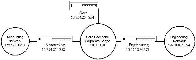
Since each ICMP error code returned has a different message, what you use depends on whether you have a specific purpose for denying the route. Considering the router setup from Example 5.2.1, what if you are in charge of the core, accounting, and engineering routers as shown in Figure 5.2.2.1? The engineering router connects to the engineering test network, 192.168.2.0/24. The accounting router connects to the accounting network, 172.17.0.0/16. All the client devices have a default route pointing to the core router, 10.254.254.254. The core router then has routes that point to the engineering, 10.254.254.253, and the accounting, 10.254.254.252, routers.
Most traffic from the main 10/8 network is not allowed onto either of these networks. The accounting network is to be administratively denied to anyone with the exceptions that the range of addresses 10.2.3.32/27 and 10.3.2.0/27 are allowed to access the accounting network. The engineering test network may be accessed by anyone on 10.10.0.0/14. All others do not even know the network exists.
This set of network security policies sounds like a firewall type of decision, but this is a common routing security structure. This is very easily done through routes on a policy router. First, you have to decide what messages you want to send back to the originating machine. In the case described above I would use the following setups for all the machines:
From accounting network - 172.17.0.0/16
10.2.3.32/27 - full route
10.3.2.0/27 - full route
10/8 - prohibit
172.16/16 - prohibit
From Engineering test network - 192.168.2.0/24
10.10/14 - full route
10/8 - blackhole
172.17/16 - blackhole
172.16/16 - blackhole
Note that these are coded in terms of "From" the respective network. This is due to the routes you are using still operating in terms of destination-based routing. Even though the types are Policy Routing, the routes themselves only code for destinations. This usage serves two purposes: First, these routes can operate on a non-Policy Routing system; second, the routing structure within the OS itself can remain streamlined in operation. As you saw in Chapter 3, the less structure placed into any one segment of the packet path, the faster the routing decision.
To apply these routes to the routers you need to consider the current connectivity of the routers. Each of the engineering and accounting routers has two interfaces: eth0 on the corporate backbone and tr0 on the respective private network. You will start from the bare system without any addressing and set up the routers.
Starting with the engineering system first you have two addresses assigned and the security policy as stated in the beginning of this example. You can set up this router in several different ways. Consider first the following command sequence:
ip addr add 192.168.2.254/24 dev tr0 brd +
ip addr add 10.254.254.253/32 dev eth0 brd 10.255.255.255
ip route add 10.10/14 scope link proto kernel dev eth0 src 10.254.254.253
Now you have added in the IP addresses and turned off the autoroute configuration for only the 10/8 network by using the /32 scope mask. Then you define a route for all traffic returning to 10.10/14 networks. The autoroute is installed for the 192.168.2.0/24 network as you wanted. Since no other routes are defined, then any other packet, such as for 172.17/16 or other 10/8 addresses, would not be routed by the system. But what happens when a router does not have a route for a packet? It will return an ICMP Type 3 Code 0, which is a "Net unreachable" message. But you do not want any errors returned to any of your other networks or to the engineering network itself. So you then add in the following routes:
ip route add blackhole 10/8
ip route add blackhole 172.17/16
ip route add blackhole 172.16/16
Now any packets that specifically try to return to any of those networks are silently dropped.
Now you consider the accounting router setup. Again you have two interfaces with addresses and the security policy statement. But in the security policy statement for this network you want to send back an ICMP Type 3 Code 13 "communication administratively prohibited" message. So you set up the accounting router as follows:
ip addr add 10.254.254.252/32 dev eth0 brd 10.255.255.255
ip addr add 172.17.254.254/16 dev tr0 brd +
ip route add 10.2.3.32/27 scope link proto kernel dev eth0 src 10.254.254.252
ip route add 10.3.2.0/27 scope link proto kernel dev eth0 src 10.254.254.252
ip route add prohibit 10/8
ip route add prohibit 172.16/16
ip route add prohibit 192.168.2/24
As noted previously, all of these routes take effect on communications that are exiting from the subnetwork. So the ICMP errors are actually returned to the systems that exist in the subnetwork itself. This is due to the routes being valid for forwarding operations only. They are destination based. When you start working with the final member of the Policy Routing triad, rules, you will see where the other packet selection mechanisms come into play.
Example 5.2.2: Multiple Routes to Same Destination
Now that you have set up the security policies using the Policy Routing route structure, you turn to the setup on the core router. Recently your company has obtained two Internet connections from two different service providers. Each connection is a T1 with an independent router and an independent assigned address scope. You want to set up load balancing for the Internet traffic.
The global information you will need is about the two different ISPs, and you will set up the multiple addresses you need on your router's external interface, eth1, as shown here:
ISP #1:
Router Interface = 1.1.1.30/27
ISP #2:
Router Interface = 2.2.2.30/27
Your router eth1 is:
ip addr add 1.1.1.1/27 dev eth1 brd +
ip addr add 2.2.2.1/27 dev eth1 brd +
Even though you have two different routes to the Internet, you would think that you can only have one default route. But you can have as many default or other routes as you would like. There are several different ways to code multiple routes to the same destination. Each method depends on the behavior you would like to have.
The first method is to use a per-packet method of multiple default routes. Under this scenario each packet entering the router will go out a different route. The main drawback to this format is that the paths to the final destination may vary in transit time enough to cause problems with packet reassembly queuing, especially with certain server types. But this is a very simple method to implement.
The route subcommand of the ip utility contains the methods allowing for multiple routers. This is coded using the equalize and nexthop commands. The nexthop command itself defines multiple gateways to send packets to and can take an optional weight command, which allows packets to be differentially balanced. The equalize command tells the route structure to send on a per-packet basis.
For example, if you decide to send each packet independently through each router, you would use the following command:
ip route add equalize default \
nexthop via 1.1.1.30 dev eth1 \
nexthop via 2.2.2.30 dev eth1
This will send each packet out through a different router. The first packet will go to 1.1.1.30, the second to 2.2.2.30, the third to 1.1.1.30, and so on ad nauseaum.
What if the router 1.1.1.30 was two T1s and the router 2.2.2.30 was a 512K fractional T1? Then you would want to weight the routes so as to send 4 packets to 1.1.1.30 for every 1 packet sent to 2.2.2.30. The easy way is to use the packet counts as weights. You would then use the following version of the command:
ip route add equalize default \
nexthop via 1.1.1.30 dev eth1 weight 4 \
nexthop via 2.2.2.30 dev eth1 weight 1
Now another way you might want to load balance is to allow each traffic flow sequence to go by one of the routes. But you do not want to inspect packets or code half the addresses one way and half the other. Instead you simply remove the equalize modifier from your multiple hop default route. Now traffic will be routed to one or the other route on a per-flow basis rather than a per-packet basis. Again you can use weights in this sense to load balance the flows themselves. Note that the per-flow is for tcp sessions while udp is treated per packet.
Example 5.2.3: Troubleshooting Unbalanced Multiple Loop Routes
You can also use the loopy routing feature to force one of the router connections to be treated as a pure input router and the other router as a pure output router. This method is often used with unbalanced connections to provide for the core site usage.
For example, suppose that you want to start providing a Web site for your corporation. You will contract with two different ISPs to provide connections. One of them will provide a T1 with a subnet of addresses for use. The other will provide 5 T1 lines with 2 IP addresses and they also agree to allow your subnet IPs from the other ISP to be sent through their connection. So you have a configuration as follows:
ISP #1:
Router 1.1.1.30/27
Subnet 1.1.1.0/27
ISP #2:
Router 2.2.2.2/30
Your usable IP - 2.2.2.1/30
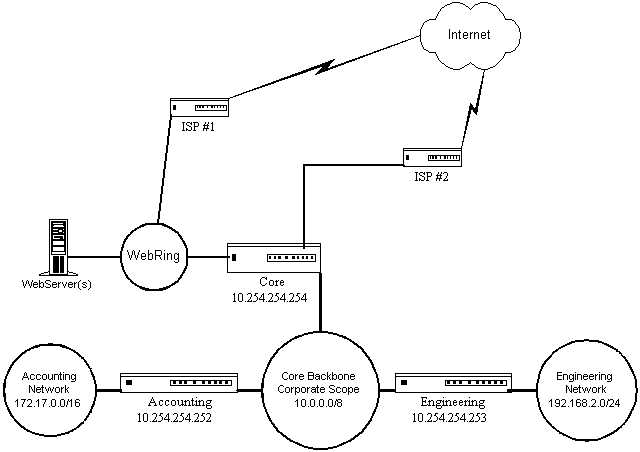
You set up a network, WebRing, to contain several Web and other Internet servers. They are assigned real IP addresses from the 1.1.1.0/27 network address space. The router from ISP #1 also connects into this network. All of your servers have a single default route pointing at your router's tr0 interface 1.1.1.1. Your other interface is connected by a crossover cable to ISP #2's router. Now the route structure is that all outgoing traffic will be routed to the Internet through ISP #2's router. Since this traffic contains the addresses given by ISP #1, the return requests will come down to your network through ISP #1's router.
Your router is not doing any real work here. The route you use simply allows all traffic from tr0 to flow out through eth0. Now your Web site gets very popular. Your notice that the uplink through ISP #2 is often running at capacity while the downlink through ISP #1 is barely cracking 256K bursts. So you decide to funnel some of the traffic through to use up some of the ISP #1 bandwidth. No problem, you simply use the weights in your router to send some traffic upward through the ISP #1 router.
And whammo, your Web site slows to a crawl. As soon as you remove the weighted routes everything is great. Upon investigation with your Ethereal brand packet sniffer you see that the Web machines are confused by the route redirects and that all the Web traffic now tries to go up through ISP #1's router.
Now you see why the placement of Policy Routing structures becomes important. In this scenario you would want to recode the default routes on the Web systems themselves to have weights. When you recode the route on your router it then informs the Web sites through a redirect to use the router from ISP #1. But since the redirect has no provision for weight, all packets then go through the ISP #1 router. When you code policy routes on the Web servers themselves, the packets are appropriately balanced and the maximum bandwidth is appropriately used.
Really the point here is that Policy Routing is not just a process for routers. Consider that many networks have servers participating in the OSPF dynamic routing protocol in order to make the routing structure simple. So too the servers should participate in the Policy Routing structure. Interestingly enough I see more usage of Policy Routing on the server in network environments today, especially where the router(s) are incapable of Policy Routing. In Chapter 6 take a hard look at the discussions of loopback routing and you will see some of the real power behind the distribution of Policy Routing structure.
If you had been assigned the block of IP addresses from ISP #1 and they were independent of the router, you could place the Web servers on a third network behind your router and you could then use the Policy Routing to balance the traffic flows. This type of setup also provides security to the systems as well and will be revisited later.
One of the topics that you have not seen is the supposed original basis for using Policy Routing in the first place - the ability to route based on source, TOS, packet data, and other packet features. This is where the final member of the Policy Routing triad, Rule, enters the scene.
As you saw in Chapter 3, rules are what provide the decision structure in the RPDB. Rules function not just as logical packet selectors, but also possess the capability to act upon a selected packet. In this sense the true power becomes apparent. Rules have much the same set of actions as routes when acting directly on a packet. Unlike routes, they cannot specify any forwarding actions but only the blocking actions. To illustrate, consider the following example.
Example 5.3.1: Basic Router Filters v2.0
Consider the setup you have running from Example 5.2.2 as illustrated by Figure 5.2.2.1. The security structure provided by the routes acts upon the traffic, leaving the subnets only. Since you have control of the core router and the subnet routers, you would like to reimplement the security structure so that the requesting client is returned the appropriate error message.
The logic revisited is that the accounting network is to be administratively denied to all except the range of addresses 10.2.3.32/27 and 10.3.2.0/27. The engineering test network may only be accessed by anyone in 10.10.0.0/14, with all others not even knowing the network exists. To summarize the logic tree:
To accounting network - 172.17.0.0/16
10.2.3.32/27 - allow
10.3.2.0/27 - allow
0/0 - prohibit
To Engineering test network - 192.168.2.0/24
10.10/14 - allow
0/0 - blackhole
Note that this logic is supposed to be from the point of view of the core router. Looking back at Example 5.2.2 you can see that the implemented logic is on the subnet routers. To ensure that your new structure is not prone to the hackery that could be done under the implementation of Example 5.2.2, you also need to look at the logic from the point of view of the subnet routers. In that manner anyone trying to subvert the global security by directly pointing at the subnet routers would be forced to obey the same rules. So the subnet router's logic would then look like:
The Accounting Network Router:
10.2.3.32/27 - allow
10.3.2.0/27 - allow
0/0 - blackhole
The Engineering test network Router:
10.10/14 - allow
0/0 - blackhole
Note that this is essentially the same as the core router logic with the exception that on the accounting router and the engineering router all traffic not allowed is silently discarded. In this manner you can essentially make the accounting and engineering routers invisible. Whether the end user workstation is coded for a default route to the core router or has entered a route directly to the accounting or engineering routers, the logical behavior of the network is consistent.
You then set about implementing this policy using the rules on the core, accounting, and engineering routers. Starting with the core router first, you allow for the default rules (see Chapter 4) and code in the following rule set:
# For the Accounting Network:
ip rule add from 10.2.3.32/27 to 172.17/16 prio 16000
ip rule add from 10.3.2.0/27 to 172.17/16 prio 16010
ip rule add from 0/0 to 172.17/16 prio 16020 prohibit
# For the Engineering Test Network:
ip rule add from 10.10/14 to 192.168.2/24 prio 17000
ip rule add from 0/0 to 192.168.2/24 prio 17010 blackhole
This allows all traffic from the allocated subnets to be passed into the routes while returning or dropping those packets not allowed. Of course you still have the routes themselves pointing to the accounting and engineering subnets. The ordering of the rules is important and you have allowed space to add rules later by spacing out the priority number. It would have sufficed to not put the "to" section in the first two rules or in the fourth. But you usually will want to err on the side of exact specification, especially when you end up placing rules into play that you come back to look at several months later. Also note that you are not specifying the interface on which the packets arrive or leave. This allows these rules to act globally. If you were certain that the traffic would be confined in transit to specific interfaces, then you would also specify the interface here. Conversely, by using an interface specification on a multi-interfaced router you can allow some traffic without having to specify any rules.
In this setup there is no restriction on any of the 10.10/14 addresses accessing the accounting network or on any of the 10.2.3.32/27, 10.3.2.0/27 addresses accessing the engineering test network. That is why you want to be able to specify Policy Routing structures on the accounting and engineering routers. By so spreading the logic, you allow for better traffic flow and also ensure that there is no one point of catastrophic failure.
You then continue on to configure the accounting router. As specified in the logic tree for Example 5.xxxxx , the accounting router will have the following rule set.
ip rule add from 10.2.3.32/27 dev eth0 prio 16000
ip rule add from 10.3.2.0/27 dev eth0 prio 16010
ip rule add from 0/0 dev eth0 prio 16020 blackhole
Note that in this case you do specify the interface on which the packets arrive. You make the assumption that if any packets originate from within the accounting network with an incorrect source address, there are other methods to deal with them.
Having coded the accounting router you turn to the engineering test network router. Again following the logic tree, you install the following rule set:
ip rule add from 10.10/14 dev eth0 prio 17000
ip rule add from 192.168.2/24 dev tr0 prio 17010
ip rule add from 0/0 prio 17020 blackhole
Now here you decide that because the engineers are wont to play with various attack programs, especially ones that use spoofing, you will limit the traffic both into and out of the network. So you allow the traffic on interface eth0 from the allowed addresses into the network. Then you allow out only the traffic with the appropriate IP address from the internal interface. Finally, you silently discard all other traffic. You essentially use the source address rules to only allow allocated addresses into and out of the network.
Note that in almost every example and discussion to this point I have not specified the type of router you are using. While the implication is that these are always Linux based systems you must bear in mind that Policy Routing is a network structure. The most common alternative to Linux for Policy Routing is Cisco's IOS router OS. With this in mind let me show you a few simple uses of Cisco Policy Routing.
The basic command for Cisco Policy Routing is the route-map command. Here is a commented example of a route-map that applies a TOS to a packet stream and then changes the next hop router.
Route-maps are applied to an interface and are named. An interface may have both inbound and outbound route maps applied. Remembering the discussion of the RPDB from Chapter 3, the first step is to select the packets of interest (match). This is done in IOS with access lists. I will select a specific IP address (10.1.1.3) for the route-map. This results in the following access list:
access-list 111 permit ip host 10.1.1.3 any
Now define the route-map named mynetmap as a general (non-directional) action on the interface of interest (in this case interface FastEthernet1/0/0)
interface FastEthernet1/0/0
ip policy route-map mynetmap
That is all for the interface configuration. This route-map does not distinguish between inbound and outbound traffic (see Cisco docs for details).
Now to define the actual route-map command and define the actions taken. Note that the number after 'permit' in the listing below is a sequence number so that additions and subtractions of actions can be made. Route-maps will always execute actions in sequence number order.
route-map mynetmap permit 10
match ip address 111
set ip tos min-delay
route-map mynetmap permit 20
match ip address 111
set ip next-hop 192.168.1.1
Note you can also do route-map mynetmap deny xx commands to forbid specific actions. Match and set conditions span the gamut of available Cisco IOS commands. These include rate limiting and traffic shaping commands as well. So the flexibility is definitely there and has been since about IOS 11.2. I strongly recommend reading through the Cisco documentation as it has many good examples and explanations.
5.5 RPDB & Multiple Route Tables
Up to this point you have been using the single master route table available within Policy Routing. All of the examples and uses have assumed that you only have a single global route structure. This is true for all known Policy Routing capable devices with the exception of Linux. At this point I will diverge into the enhanced world of Policy Routing structures under Linux.
As you saw in Chapter 3, within the Linux Policy Routing structure there is provision for 255 independent routing tables. The standard structure allocation provides a default structure. Recalling this information from Chapter 3 and Chapter 4, you have the following default table structure:
Table #253 = DEFAULT (created by the default rule #32767)
Table #254 = MAIN (default master route table)
Table #255 = LOCAL (broadcast & local addresses)
As you recall from Chapter 3, of these tables the LOCAL table should not be modified or used normally. It has a special functionality with respect to the broadcast and local route structures.
The naming of these tables is handled by a lookup reference file. This file is /etc/iproute2/rt_tables. While you can always reference the tables by number from 1-255, it is easier to read your scripts if you name the tables. I usually will place a comment at the beginning of my scripts that states the names and numbers association so that the file still makes sense if someone changes the rt_tables mapping.
Example 5.5.1: Basic Router Filters v3.0
In order to use the flexibility immediately accorded to you by the specification of multiple routing tables, you decide to recode your security structure from Example 5.3.1 in terms of simpler rules. You start with the core router. You decide to create two new route tables that contain the routes for the accounting and engineering networks. First you edit the rt_tables file and name the tables appropriately as follows:
# reserved values
#
255 local
254 main
253 default
0 unspec
#
# Policy Routing Example 5.5.1
#
1 accounting
2 engineering
#
# end rt_tables
Now you start to populate the route tables and rules.
Note that the specification of the complete routing and security structure can now be fulfilled on the core router. In Example 5.xxxx you were limited because of the rules. In that setup any traffic selected for either the engineering or accounting network could be routed to the other network. IE: Any traffic from 10.10/14 could be routed to the accounting network due to being selected for fall through to the main table by the Engineering rule. And vice versa, the Accounting-allowed rule traffic would fall through to the main table and could be routed to the engineering network.
Now you see that you can specify exactly that all traffic to either of these networks be segregated into a table by the appropriate rule. Thus you only need three rules to specify all the traffic flow. You need to create the rules first by starting fresh on the core router without any routes or rules referring to the accounting or engineering networks.
# For the Accounting Network
ip rule add from 10.2.3.32/27 to 172.17/16 prio 16000 table accounting
ip rule add from 10.3.2.0/27 to 172.17/16 prio 16010 table accounting
# For the Engineering Test Network
ip rule add from 10.10/14 to 192.168.2/24 prio 17000 table engineering
This sends the traffic destined for the respective network to a route table for that network, and only such traffic will get to the table. Now you need to code the accounting and engineering route tables.
# The accounting table #1
ip route add 172.17/16 table accounting via 10.254.254.252 proto static
ip route add prohibit default
# The engineering table #2
ip route add 192.168.2/24 table engineering via 10.254.254.253 proto static
ip route add blackhole default
Now all traffic flowing to the these networks is segregated and you have implemented the security policy. Or have you?
Recalling that the original security policy stated that all traffic to the accounting network that was not permitted was to be returned an ICMP Administratively Denied message and that no one was to be able to determine that the engineering test network existed if they were not permitted to access it. Does this setup still follow those maxims? Upon further inspection you determine that it does not. Why?
You added in to the accounting and engineering routing tables default routes that specified the appropriate actions to take. For accounting you prohibit and for engineering you blackhole. But what if someone from the 10/8 network who is not allowed onto engineering, in other words someone sourced outside 10.10/14, decides to try to get to 192.168.2/24? From the rules above they would end up in the main table. Now the main table does not have a route to the engineering network so that by default the router will return a ICMP Network Unreachable. This is not the same as a blackhole where the packets are dropped. So the default route in the engineering table is never reached or used. Ditto for the accounting network.
The trick then is to still use the rules to control the flow of alternate traffic. You do note that you had purposely allocated space in the rule priority selection so that you could also insert rules later on. To complete the Policy Routing structure, you add in the rules to control the unwanted traffic streams:
# For Accounting network
ip rule add from 0/0 to 172.17/16 prio 16050 prohibit
# For Engineering test network
ip rule add from 0/0 to 192.168.2/24 prio 17050 blackhole
Now you have the security policy completely specified on the core router. Turning to the accounting and engineering routers you see that the setups as specified in Example 5.3.1 are sufficient for the current security structure.
At this point you review the total Policy Routing structure. The core router has the main role in the routing structure. It provides the appropriate error messages and allowed traffic control to the accounting and engineering networks. This policy structure is supported by the implementation on the accounting and engineering routers. These subnetwork routers reinforce the security policy by allowing only the traffic that is allowed. While in this type of setup you could have dispensed with implementing any policy on the core router, you want to stress that the core router should always be the default. The subnetwork routers merely prevent internal hackery.
You can see how without the multiple routing tables on the core router you would not have been able to lock down the traffic to the subnetworks as accurately. This is true of many situations in Policy Routing. Since each routing table is completely independent of the others, there can be no crossover bleed of misdirected routes.
Having tackled the setup required for implementing this Policy Routing structure you want to move on to bigger projects. Luckily you have been selected to assist in incorporating a recently acquired company into the corporate network fabric.
This company has three different connections into the core network:
The first connection is the Internet and is mediated from an existing
firewall you have no control over.
The second connection is the primary vendor who has provided a
connection to their ordering system.
The third connection is the primary transport supplier who has
provided a connection into their scheduling system.
The network connections all terminate into a single Token Ring network. Currently there are four small Token Ring-Ethernet routers installed between the internal Ethernets and the Token Ring. Additionally, there is a translating bridge between the two Ethernets and the Token Ring for the Internet connection. Your job is to fix and secure this mess.
The networks and connections from the three outside networks are shown in Listing 5.6.1.
Listing 5.6.1 All Together Now Initial Notes
Internet
Allocated DMZ Address Space from Firewall: 172.16.1.0/24
Firewall TokenRing Interface: 172.16.1.254, 192.168.1.254, 192.168.2.254
Provides NAT for all addresses in the 192.168.0/22 range
Vendor1
Allocated DMZ Addresses: 192.168.100.0/24
Router TokenRing Interface: 192.168.100.254
Provides Connection to 172.18/16
Allows routes to 192.168.1/24 and 192.168.2/24
Supplier1
Allocated DMZ Addresses: 192.168.200.0/24
Router TokenRing Interface: 192.168.200.254
Provides Connection to 10.10/16
Allows routes to 192.168.1/24 and 192.168.2/24
You find out the the two internal Ethernets use 192.168.1.0/24 and 192.168.2.0/24. Now some of the allowances from the routers make sense. Digging further you find out that only some people are supposed to be allowed into either or both of the Vendor and Supplier networks. And there are several groups of computers that management would like to not have Internet access.
You write down all of the information and distill it into Listing 5.6.2.
Listing 5.6.2 All Together Now Routing/Security Policy
Allowed to Vendor network
192.168.1.0/24
192.168.2.32/27
Allowed to Supplier network
192.168.2.0/24
192.168.128/29
Denied Internet
192.168.1.128/25
192.168.2.32/27
Fairly simple so far. You take out all four small routers and both of the translating bridges so that nothing now connects the TokenRing with the internal Ethernets. You decide to use a single Policy Routing core router between the internal Ethernets and the Token Ring DMZ. While determining where to install the Ethernet cables you discover that the two Ethernets are actually only two different hubs with a backplane connection, thus making them one physical network thus you only need one physical Ethernet interface. Well, this will be even easier you think, hoping that nothing else pops up to surprise you.
You start configuring your core router by notating the addresses and primary routes as in Listing 5.6.3.
Listing 5.6.3 All Together Now Address & Routes Notes
# tr0
172.16.1.1/24
192.168.100.1/24
192.168.200.1/24
# eth0
192.168.1.254/24
192.168.2.254/24
# Primary Routes
172.18.0.0/16 through gateway 192.168.100.254 (Vendor)
10.10.0.0/16 through gateway 192.168.200.254 (Supplier)
Default through gateway 172.16.1.254 (Internet)
You now have both your configuration and your security policy. You now decide to create one script to implement the corresponding Policy Routing structure. This script with comments is shown in Listing 5.6.4.
Listing 5.6.4 All Together Now - The Script
# Begin script for CORPALL V1.0
#
# Vendor Net: 172.18/16 / router 192.168.100.254/24
# Supplier Net: 10.10/16 / router 192.168.200.254/24
# Internet Firewall: default / router 172.16.1.254/24
#
# Implement Multiple IP Addresses
#
# TokenRing 0 - DMZ
ip addr add 172.16.1.1/24 dev tr0 brd +
ip addr add 192.168.100.1/24 dev tr0 brd +
ip addr add 192.168.200.1/24 dev tr0 brd +
#
# Ethernet 0 - Internal Ethernets
ip addr add 192.168.1.254/24 dev eth0 brd +
ip addr add 192.168.2.254/24 dev eth0 brd +
#
# Implement Routing Tables
# Table 1 = vendor
# Table 2 = supplier
# Table 3 = inet
#
# To Internet - use inet table
ip route add default via 172.16.1.254 proto static table inet
#
# To Vendor Net - use vendor table
ip route add 172.18/16 via 192.168.100.254 proto static table vendor
#
# To Supplier Net - use supplier table
ip route add 10.10/16 via 192.168.200.254 proto static table supplier
#
# Implement Rules
# 15000 - 15999 use for Vendor
# 16000 - 16999 use for Supplier
# 17000 - 17999 use for Internet
#
# To Vendor Net
ip rule add from 192.168.1.0/24 to 172.18/16 prio 15000 table vendor
ip rule add from 192.168.2.32/27 to 172.18/16 prio 15100 table vendor
#
# To Supplier Net
ip rule add from 192.168.2.0/24 to 10.10/16 prio 16000 table supplier
ip rule add from 192.168.1.128/29 to 10.10/16 prio 16100 table supplier
#
# To Internet
ip rule add from 192.168.1.0/25 to 0/0 prio 17000 table inet
ip rule add from 192.168.2.0/27 to 0/0 prio 17100 table inet
ip rule add from 192.168.2.64/26 to 0/0 prio 17200 table inet
ip rule add from 192.168.2.128/25 to 0/0 prio 17300 table inet
#
# Force Policy Routing Structure Update
ip route flush cache
#
# end CORPALL version 1.0
You can then run this configuration script on your Policy Routing core router and you will have a complete implementation. This one script ties together all of the parts of basic Policy Routing implementation. You have multiple IP addresses, multiple routing tables, rules, and a defined structure for implementation.
Just to prove to yourself that this is not the only way to implement this structure, you create an alternate script as in Listing 5.6.5.
Listing 5.6.5 All Together Now - The Other Script Upon careful study, you determine
that this script would also correctly implement the Policy Routing
structure you want. The first script used three additional routing
tables and simple rules. The second script uses only one additional
table and more complex rules. But both will work identically from the
point of view of the traffic through the router. You now have your black belt in
basic Policy Routing implementation. You see from the final example
that there is usually more than one correct implementation method.
You see how the Triad elements of Policy Routing, Address, Route, and
Rule, support, intermingle, and interact with each other. You are now ready to start
considering the advanced implications of Policy Routing structures.
You wonder how the core triad interacts with other network
structures. Especially when you start considering dynamic routing,
NAT, firewalling, QoS, and packet filters. These subjects are the
next you start to study as you begin to see the larger network
picture emerge.
# Begin script for CORPALL V1.0 Alternate
#
# Vendor Net:
# 172.18/16 / router 192.168.100.254/24
# Supplier Net:
# 10.10/16 / router 192.168.200.254/24
# Internet Firewall:
# default / router 172.16.1.254/24
#
# Implement Multiple IP Addresses
#
# TokenRing 0 - DMZ
ip addr add 172.16.1.1/24 dev tr0 brd +
ip addr add 192.168.100.1/24 dev tr0 brd +
ip addr add 192.168.200.1/24 dev tr0 brd +
#
# Ethernet 0 - Internal Ethernets
ip addr add 192.168.1.254/24 dev eth0 brd +
ip addr add 192.168.2.254/24 dev eth0 brd +
#
# Implement Routing Tables
# Table 1 = external
#
# To Internet - use main table default route
ip route add default via 172.16.1.254 proto static
#
# To Vendor Net - use external table
ip route add 172.18/16 via 192.168.100.254 proto static table external
#
# To Supplier Net - use external table
ip route add 10.10/16 via 192.168.200.254 proto static table external
#
# Implement Rules
# 15000 - 15999 use for Vendor
# 16000 - 16999 use for Supplier
# 17000 - 17999 use for Internet
#
# To Vendor Net
ip rule add from 192.168.1.0/24 to 172.18/16 prio 15000 table external
ip rule add from 192.168.2.32/27 to 172.18/16 prio 15100 table external
ip rule add from 0/0 to 172.18/16 prio 15999 table external blackhole
#
# To Supplier Net
ip rule add from 192.168.2.0/24 to 10.10/16 prio 16000 table external
ip rule add from 192.168.1.128/29 to 10.10/16 prio 16100 table external
ip rule add from 0/0 to 10.10/16 prio 16999 table external blackhole
#
# To Internet
ip rule add from 192.168.1.128/25 to 0/0 prio 17000 table main blackhole
ip rule add from 192.168.2.32/27 to 0/0 prio 17100 table main blackhole
#
# Default AntiSpoof
ip rule add from 192.168.1.0/24 to 0/0 dev eth0 prio 17200
ip rule add from 192.168.2.0/24 to 0/0 dev eth0 prio 17300
ip rule add from 0/0 dev eth0 prio 17999 blackhole
#
# Force Policy Routing Structure Update
ip route flush cache
#
# end CORPALL version 1.0 Alternate